MATERIAL

The shells of Margaritifera margaritifera (Linnaeus, 1758) were originally collected from their life habitat in northern Finland. Three shells of M. margaritifera were collected alive in late autumn of 2002 from their life habitat under the license from the North Ostrobothnia Regional Environment Centre during the fieldwork for the WWF project (Valovirta et al. 2003). The shells now belong to the invertebrate collections of the Finnish Museum of Natural History, University of Helsinki, from which they were retrieved for this study. The lengths of the specimens H1, H2 and H3 varied between 80 and 98 mm.

ENVIRONMENTAL SETTING

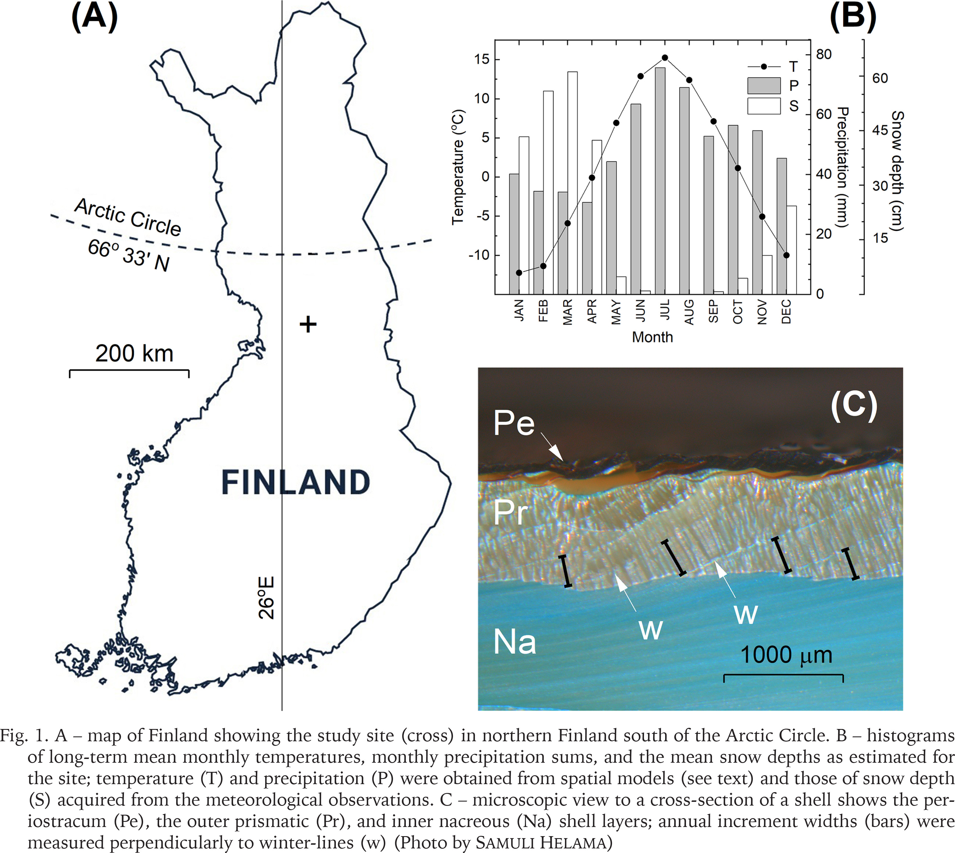
Our study site is located in northern Finland (Fig. 1A), approx. 125 km south of the Arctic Circle, in the region characterised by both the north and middle boreal forests (Ahti et al. 1968) typically dominated by unmanaged and managed stands of Norway spruce, birch and Scots pine. The life habitat of the bivalves, the stream of Haukioja, is an approx. 10 km long and narrow (2–3 m) rivulet that meanders through mineral terrains and peatlands, with a fall of approx. 70 m. The bottom of the stream is sandy, with pebbles and boulders. According to Hyvönen et al. (2005), the stream has been disturbed by forestry operations and the manmade ditches have resulted in the growing surplus of sand in the stream bottom habitat. Local (unpublished) forestry archives show that ditching of the forest land have taken place in the vicinity of the habitat mainly between the years 1985 and 1988 (A. Kuvaja, pers. comm.). The climate of the region is characterised by distinct seasons (Fig. 1B), with annual mean temperature around +1 °C and annual precipitation sum around 600 mm. The snow season starts in October/November and lasts until April/May.

Fig. 1

A – map of Finland showing the study site (cross) in northern Finland south of the Arctic Circle. B – histograms of long-term mean monthly temperatures, monthly precipitation sums, and the mean snow depths as estimated for the site; temperature (T) and precipitation (P) were obtained from spatial models (see text) and those of snow depth (S) acquired from the meteorological observations. C – microscopic view to a cross-section of a shell shows the periostracum (Pe), the outer prismatic (Pr), and inner nacreous (Na) shell layers; annual increment widths (bars) were measured perpendicularly to winter-lines (w) (Photo by Samuli Helama)

ANNUAL SHELL GROWTH INCREMENTS

Although the growth bands of bivalve may be visible on the shell surface, the internal growth lines (which correspond to the external growth lines) can be identified from carefully prepared cross-sections and provide more reliable results on bivalve growth and age (Andrzejewski et al. 2012, Eszer et al. 2016). Cross-sections of M. margaritifera shells display distinct annually formed increments, as demonstrated by Dunca et al. (2005), who studied the annual increments of this species in southern Sweden. They showed that while shell growth starts in May and ends in October, it ceases during the cold season with formation of ‘winter lines’, which provide the framework for identification of annual increments and, accordingly, the sclerochronological analyses. Following their recommendations, the shells of our study were cut from umbo to the ventral margin and cross-sections were ground and polished manually, and etched in the Mutvei’s solution at 37–40 °C for ca. 25 min (Mutvei et al. 1996, Schöne et al. 2005). Annual increment widths were measured from the cross-sections of the outer shell layer, to the nearest 1 μm, perpendicular to the ‘winter lines’ from digital images that were photographed by an Olympus DP10 camera attached to an Olympus BX40 microscope (Fig. 1C).

Sclerochronological cross-dating was carried out to ensure that no false increment was included in any of the samples and that no increment had been accidentally missed. This comparison was first performed between the growth records of left and right valves of each individual bivalve, to detect any potential offsets in the samples. As a second step, the series of left and right valves were averaged, and the arithmetic mean series of different individuals were similarly compared for their growth synchrony.

Annual shell growth increments of M. margaritifera are known to contain non-climatic trends during ontogeny that should be eliminated from the series prior to statistical inquiries (e.g. Dunca 1999). Such a detrending was carried out here by fitting a curve in the form of a modified exponential function (Fritts 1976) to each series. Dimensionless indices were extracted by dividing the actual increment width value by the value expected by the curve. Mean chronologies representing growth variability of each individual were produced by averaging the index values from left and right valves. These average series were used to calculate a final mean chronology representing growth variations at the site. Arithmetic mean was used for these calculations, the calculations following the routines applied in the context of tree-ring research (Fritts 1976).

CHRONOLOGY STATISTICS

As a measure of the strength of the common growth ‘signal’ within the chronology and to estimate chronology reliability, Pearson correlations between the index series were calculated (Briffa & Jones 1990). Expressed population signal (EPS) was used as indication of chronology reliability and to measure the expression of common variability among the available growth series. Following Wigley et al. (1984), the criterion of EPS > 0.85 was considered as a reasonable (albeit objective) value for an acceptable level of chronology confidence. Cook & Pederson (2011) provided formulae to calculate the EPS-statistic for a dataset with multiple tree-ring index series per sampled tree. Here, we used these formulae as presented by Cook & Pederson (2011) to calculate the same statistic for a sclerochronological dataset with data from both valves of each shell specimen. The period 1976–2002, when the shell growth increment chronology was covered by all the index series, was used for these and the subsequent (see next paragraph) analyses.

CLIMATIC CORRELATIONS

The climatic variables that had affected the shell growth were revealed using linear (Pearson) correlations. Correlation coefficients were computed between the mean chronology and the series of monthly temperature and precipitation variables. The climatic data for the life habitat of our bivalves were obtained from the spatial model built using the monthly mean temperatures and monthly precipitation sums collected by the Finnish Meteorological Institute. The model was built by Aalto et al. (2013, 2016) using kriging interpolation to account for the influence of topography and water bodies. The estimates of Aalto et al. (2016) contain snow data only for the 2016–2020 period, for which reason a maximum snow depth record was obtained as the mean series of Kurenalus and Jaurakkajärvi meteorological stations, which are located ~30 km west and ~20 km south of our site, respectively. The means and standard deviations of Kurenalus and Jaurakkajärvi snow records were different. Therefore, before averaging, the mean and standard deviation of the Jaurakkajärvi record were set to equal those of Kurenalus record. We used the maximum snow depth as this variable was previously connected to shell growth of riverine bivalves (Watanabe et al. 2021).

Sclerochronological records may be autocorrelated (Reynolds et al. 2022), which means that the statistical significance cannot be evaluated by referring to standard tables. In order to circumvent this problem, the significance of the correlations was evaluated using a combination of frequency-domain modelling (Ebisuzaki 1997) and Monte Carlo (Efron & Tibshirani 1986) methods. One thousand (1,000) pairs of surrogate timeseries with the same power spectrum as the original series but with a random phase were generated and correlated with each other. This led us to determine the empirical probability distribution of the statistic and, accordingly, to assess the significance for similarly autocorrelated timeseries from the two-tailed distribution (Macias-Fauria et al. 2012). Shell growth, represented by the chronology of six valves, was explained by a climatic variable, using linear regression. In addition to statistical hypothesis testing, Johnson (1999) emphasised the value of estimating confidence intervals for determining the importance of factors. Confidence intervals for the model were calculated, following Macias-Fauria et al. (2010), based on 1,000 surrogate series of residuals generated with the same autocorrelation structure (Burg 1978) as the residuals from the original linear regression. The t-residuals (Graybill & Iyer 1994) from the regression were plotted. According to Graybill & Iyer (1994), the absolute value of t greater than 2.0 could be taken as an indication of a potential outlier. The test of Durbin & Watson (1951) was used to examine serial correlation in the model residuals.

CROSS-DATING

The specimen H1 contained a higher number of annual increments than any of the remaining specimens (Fig. 2A). The first observable increment in H1 was formed in 1966, whereas the corresponding increments in other specimens were dated to 1976, in both H2 and H3 (Fig. 2B–C). However, the first increment in the right valve of H3 was dated to 1977. Hence, the mussels were at least 27–37 years old when sacrificed.

Fig. 2

Annual shell growth increment records: A–C – comparison between the series of left (L) and right (R) valves of the specimens H1, H2 and H3; D – comparison between the series of specimen H3 after a microscopic reinvestigation

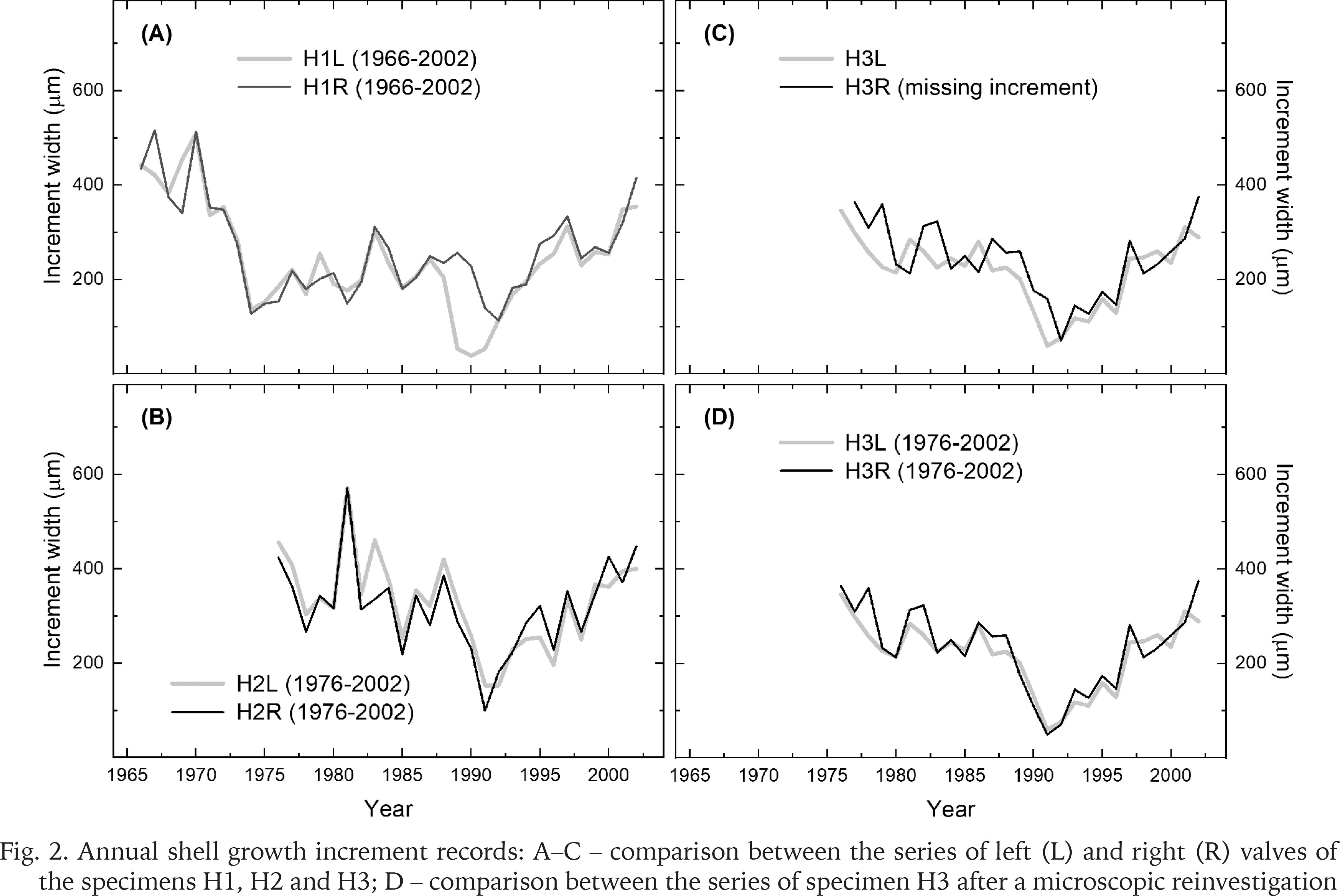
All the increment series showed decline in width over the first ten to fifteen years (Fig. 2). Another common pattern was the increase in shell growth since the early 1990s. In this regard, the growth variations were very similar in left and right valves, with two exceptions. First, the left valve of the specimen H1 showed a phase of growth curtailment in 1989–1990, that is, during the years predating the phase of low growth in its right valve (Fig. 2A). Second, it appeared that prior to the 1990s, the growth patterns based on left and right values of the specimen H3 were offset by a year (Fig. 2C). Reinvestigation of the cross-sections revealed that one annual increment (that of 1991) had been accidentally missed in the sample H3R. As a result, the remeasured series of the specimen H3 did not indicate any offset between the left and right valves (Fig. 2D).

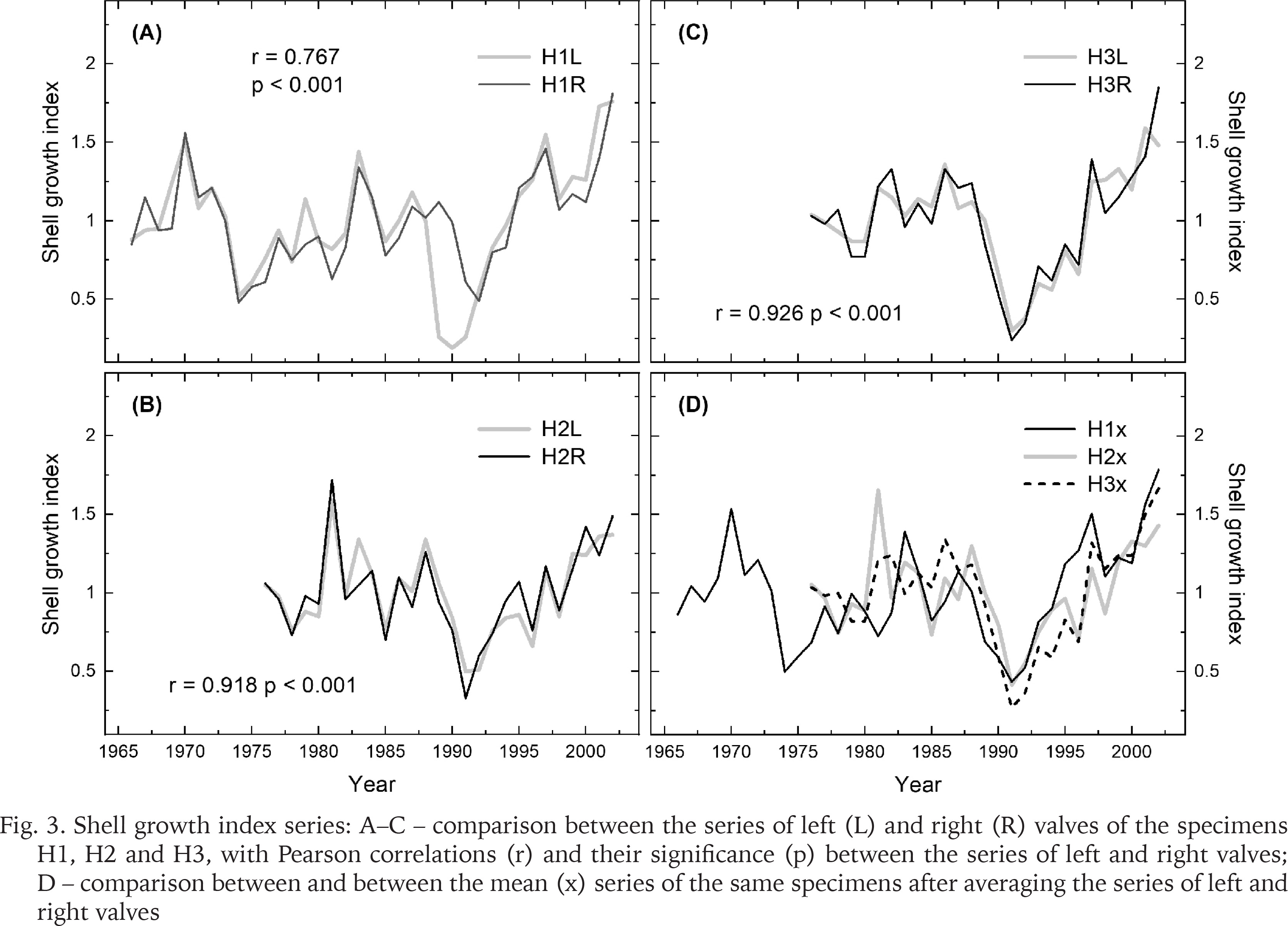
The growth indices portrayed the annual variations in shell growth on inter-annual to longer scales (Fig. 3). A feature common to all the series was the drop in shell growth in 1991 in most of the series, and the growth release postdating that event. Comparing visually the series from left and right valves of each individual (Fig. 3A–C), and the series of different individuals (Fig. 3D), illustrate less similar growth patterns between the mussels than between the valves. Even so, the series of individual mussels were clearly correlating with each other. A year with contrasting growth pattern was, however, observed in 1981 when the oldest individual (H1) did not indicate such high growth values as in the two other mussels.

Fig. 3

Shell growth index series: A–C – comparison between the series of left (L) and right (R) valves of the specimens H1, H2 and H3, with Pearson correlations (r) and their significance (p) between the series of left and right valves; D – comparison between and between the mean (x) series of the same specimens after averaging the series of left and right valves

THE EPS-STATISTIC

Confirming the visual comparisons, highest correlations (r) were evident for the index series based on left and right valves of the individuals, these correlations averaging r = 0.860 (Fig. 4). In comparison, correlations between the valves of different individuals averaged r = 0.631. Averaging the series of left and right valves for each individual bivalve marginally increased the correlation, the Pearson correlations among these mean series averaging r = 0.681.

Fig. 4

Sclerochronological correlations. Mean (Pearson) correlation within (w/i) each individual calculated between the shell growth index series of same individuals’ left and right valves; mean correlation of valves between (b/w) the different individuals; and mean correlation for the mean series that were averaged (avg) from the left and right valves

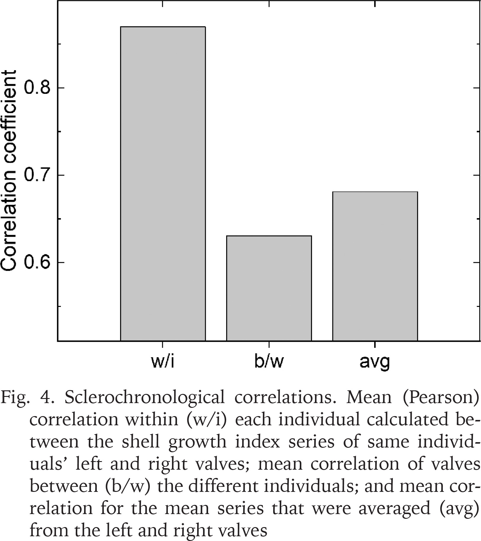
The EPS-statistic for the chronology of six valves was 0.864. This figure exceeded the criterion of EPS > 0.85 that is generally considered an acceptable level of chronology confidence (Wigley et al. 1984). Had we used only left or right valves of each specimen, the EPS = 0.837 would have been obtained. This figure was calculated by adopting r = 0.631 (see above), that excludes the correlations between the series of individuals’ left and right valve.

CLIMATIC RELATIONSHIPS

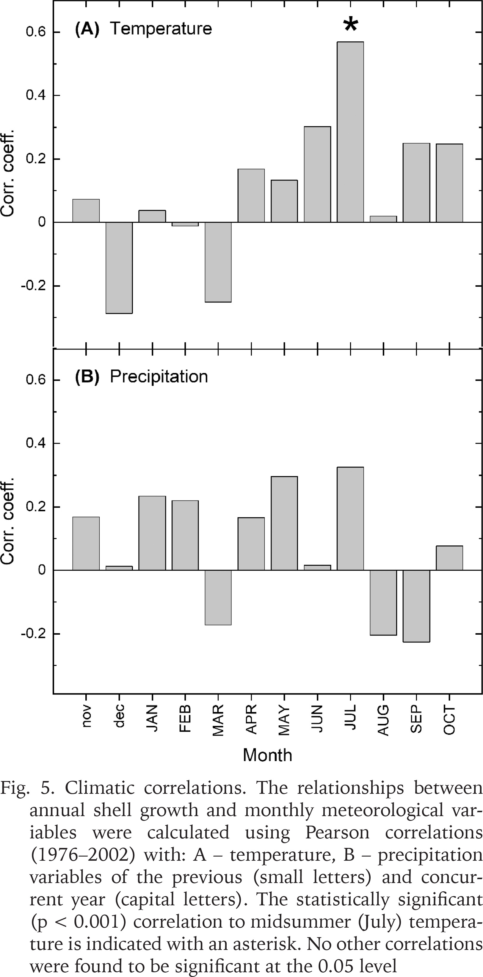
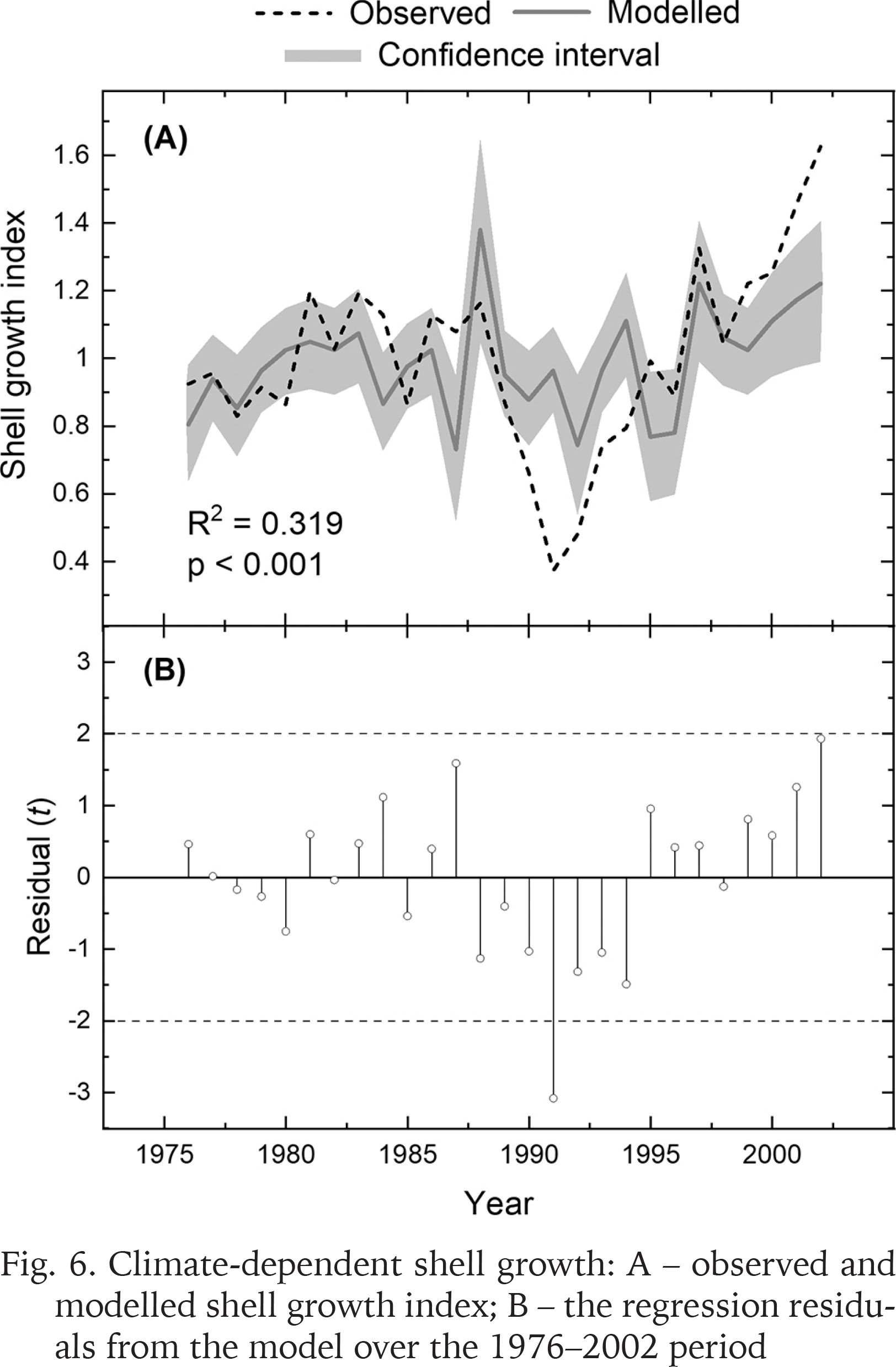
Correlations with climatic records indicated that shell growth variability was predominantly related to summer temperatures (Fig. 5). The climate-growth correlations calculated for the 27-year period (1976–2002) showed that shell growth responded markedly positively to temperatures in June and July (Fig. 5A). However, the midsummer (July) temperature was the only variable correlating statistically significantly (p < 0.001) with shell growth. Precipitation variables did not exhibit statistically significant correlations with shell growth (Fig. 5B). Correlating the shell growth chronology with maximum snow depth over the same interval resulted in a non-significant correlation of r = 0.167. Linear regression was used to explain shell growth variations by July temperatures (Fig. 6A). The temperature variable explained approx. one third of the variance in shell growth, as can be seen from R² = 0.319. Durbin-Watson–statistic d = 1.922 implied that the residuals were not statistically significantly (0.01 level) autocorrelated. The residuals from the regression were negative between the years 1988 and 1994, and predominantly positive since then (Fig. 6B). This means that the statistical model overestimates the growth level over the 1988–1994 period when the observed growth lies outside the confidence intervals of the growth model. However, the growth seems to have increased somewhat faster than the model predicted during the early years of the 2000s. In any case, the residuals exhibited |t| >2.0 for one calendar year (1991), an indication of a potential outlier.

Fig. 5

Climatic correlations. The relationships between annual shell growth and monthly meteorological variables were calculated using Pearson correlations (1976–2002) with: A – temperature, B – precipitation variables of the previous (small letters) and concurrent year (capital letters). The statistically significant (p < 0.001) correlation to midsummer (July) temperature is indicated with an asterisk. No other correlations were found to be significant at the 0.05 level

Fig. 6

Climate-dependent shell growth: A – observed and modelled shell growth index; B – the regression residuals from the model over the 1976–2002 period

BUILDING THE CHRONOLOGY

It appears common that either left or right valves are chosen for sclerochronological analyses. This may be a fair point for assemblages where shells are disarticulated or for species with asymmetrical valves. In some studies, both valves of one specimen may have been analysed for experimental purposes for illustrating the ‘intra-reproducibility’ of the analysis (Doré et al. 2020). Here we have taken an alternative approach. We have found that analysing both valves of Margaritifera margaritifera come with some benefits for sclerochronological investigations, compared to analyses of single valves. First, comparing the shell growth records of left and right valves provided means to check that the measurements contain no mistakes. That is, cross-matching between the two growth records of the same individual helps confirm that no increments have been missed or falsely added in the growth records of that individual, before comparing the records of different bivalves. This step of cross-dating process mimicked that of ‘intra-shell cross-dating’, as previously demonstrated for a marine bivalve Arctica islandica (Helama & Hood 2011). In their approach, the annual shell growth increment records were produced separately from hinge plate and shell margin, after which the two series of the same individual were cross-matched against each other, prior to any cross-dating between similarly generated records of Arctica islandica bivalves.

Second, the EPS-statistic computed for our M. margaritifera chronology (0.86) exceeded the threshold of 0.85, which is generally considered an acceptable level of chronology confidence (Wigley et al. 1984). Further, it could be calculated that the use of only one valve from each specimen had resulted in an EPS value below the foregoing criterion. These findings bear implications for shell collections needed to build a statistically robust sclerochronological dataset. The studied species, M. margaritifera, has been included in The IUCN Red List of Threatened Species (Moorkens et al. 2017). This means that the number of shells collected alive even for research purposes should be kept down. Our findings contribute to this aim by showing that an acceptable level of EPS-statistic can be reached with a lower number of individual bivalves when both valves are investigated and used to build the chronology. Apart from sample size, the EPS-statistic is affected by the correlations among the growth series, for which reason global guidelines on sample size requirements cannot be provided. Correlations among the growth records vary between the populations (Rypel et al. 2008, 2009, Black et al. 2010, 2015), as a function of time (Watanabe et al. 2021, Reynolds et al. 2022) and geographical distance (Marchitto et al. 2000, Butler et al. 2009). The correlations are also affected by method used to detrend the original increment records (Helama et al. 2006). Our results show that the correlations also depend on whether the series originate from different valves of the same individual or from different individuals (Fig. 4). According to the terminology of Hurlbert (1984), increased replication reduces the effects of “noise” or random variations or error, thereby increasing the precision of our growth estimates. The use of one site chronology from multiple valves, however, represents pseudoreplication which may give false impression of a larger number of degrees of freedom, inflating p-values if not correctly counted for. In this regard, we emphasise the importance of using the EPS formulae tailored for those datasets that contain multiple growth series per individual (Cook & Pederson 2011). Since the correlations among multiple series of one individual were higher than those between the bivalves, including those values in standard EPS equations (Wigley et al. 1984, Briffa & Jones 1990, Briffa 1995, Buras 2017) could inflate the EPS results, leading to overly optimistic estimates of chronology confidence.

Third, the growth values of right valve of the specimen H1 were markedly lower in 1989 and 1990, over which years no similar growth curtailment was evident in any other growth record (Fig. 2A and 3A). One possible explanation for the observed growth anomaly may be a shell injury, that may have in this case affected only one of the valves. The anomalous growth was recovered in less than five years, in which interval the growth of the affected valve reached the growth level of unaffected (left) valve. Similar timespan of shell repair, from five to eight years after the injury, has been previously illustrated for M. margaritifera shell growth (Helama & Valovirta 2008a). Overall, these comparisons demonstrate the potential of using the sclerochronological cross-dating to analyse short-term anomalies in bivalve shell growth.

An unavoidable disadvantage of our approach is that both valves of the studied bivalves are processed and prepared for cross sections by cutting them, for which reason there will be no extra valves remaining as intact. This may be particularly relevant if intact specimens are later needed for research purposes of which necessity could not have been anticipated when the sclerochronological analysis was carried out.

CLIMATIC AND HYDROLOGICAL FACTORS

Previous riverine studies have related sclerochronological data to hydrological factors. In the US Southeast (Mississippi, Arkansas, Alabama), annual shell growth increments of several species correlated negatively to mean annual streamflow (Rypel et al. 2008), annual flood pulse count, and May and June discharge (Rypel et al. 2009). Similar (negative) correlations have also been found for shell growth of several freshwater bivalves and river discharge in the Pacific Northwestern streams (Black et al. 2010, 2015). In Hokkaido (Japan), the shell growth of Margaritifera laevis was negatively correlated with maximum snow depth, the latter variable being closely related to the average water discharge in May (Watanabe et al. 2021). Collectively, these studies indicate that the riverine species are impaired by increased flow pulses typical to spring or early summer. Similar relationships could not be confirmed by our results. That is, the correlation between maximum snow depth and shell growth remained statistically non-significant. Moreover, the correlation between the shell growth and January precipitation, which acts as a reasonable predictor of January–March snow depth in northern Finland (Helama et al. 2013), was also non-significant (Fig. 5B).

Apart from these natural determinants, shell growth showed a negative excursion between the years 1988 and 1994 (Figs 2–3) that could not be fully explained by the climatic model (Fig. 6). Here, we refer to Hyvönen et al. (2005) who have documented a compound disturbance of the studied stream by forestry operations and manmade ditches that have resulted in a growing surplus of sand in the stream bottom habitat, as well as to the information that these forestry operations were particularly active over the 1985–1988 period. Intriguingly, the start of the negative growth event in 1988 and its continuation over the subsequent years would point to a lagged, nearly decadal period of deteriorated bivalve growth. It is known that M. margaritifera actively emigrate from sand-dominated microhabitats, suggestively to avoid dislodgment from such hydraulically unstable habitats, while remaining more sedentary in gravel- or stone-dominated microhabitats (Eissenhauer et al. 2023). With the information we have gathered, we conclude that the growth curtailment was most likely caused by the increased influx of clastic sediments in the stream due to anthropogenic changes in the catchment. Even so, it remains possible that also the food quality was affected, given that the anthropogenic changes increased the proportion of terrestrial-based detritus in river water. Feeding experiments with juvenile M. margaritifera show that such food type results in markedly lowered growth rates (Grunicke et al. 2023). Combined, this interpretation concurs with the multiple stressor framework (Kuglerová et al. 2021) compiled for estimating the negative local-scale effects from forestry activities on macroinvertebrates in Swedish and Finnish streams.

In addition to hydrological conditions, shell growth variability was related to summer temperatures. This finding agreed with previous sclerochronological M. margaritifera studies where similar warm-season relationships have been demonstrated for several riverine sites in Sweden (Dunca 1999, Schöne et al. 2004, Dunca et al. 2005) and northern Finland (Helama et al. 2009a, 2010, Helama & Valovirta 2014). Compared to these studies, the seasonal window of statistically significant correlation we found was more limited and related only to midsummer (July) temperatures (Fig. 5A). That only summer temperature was found to influence the shell growth concurs with indications that anomalous thermal conditions in winter may not impair M. margaritifera, as observed at least for the juveniles of the species (Wagner et al. 2024). These findings could suggest that the thermal constraints of summer season remain the most important factor for the species in the studied habitat.

Our findings are based on one site chronology which means the results should not be straightforwardly extended to other streams and habitats. Moreover, longer growth records would be needed to elaborate the relationships and to detail their potential time and timescale-dependent characteristics (Helama & Valovirta 2014). In Finland, sclerochronological analyses have been successfully carried out using dead-collected M. margaritifera shells (Helama et al. 2007, 2009a, 2009b, 2010, Helama & Valovirta 2007, 2008a, 2008b, 2014, Helama & Nielsen 2008). Complying with the benefits of conservation paleobiology (Flessa 2002, Dillon et al. 2022), this approach does not reduce the number of potentially reproducing individuals in the extant populations. As a future prospect, similar approach could possibly be applied to extend the existing shell increment chronology of the studied stream, both back in time and toward the present, using the shells collected from their death assemblages. The data produced in this study can be used in such analyses. The motivation for such an extension of the chronology comes from the possibility to investigate the growth and vitality of M. margaritifera in long-term perspective before and after the observed anthropogenic event, to understand the requirements and vulnerability of this endangered species in its natural and disturbed life habitats.